Partitioning

Clearly, we must break away from the sequential and not limit the computers. We must state definitions and provide for priorities and descriptions of data. We must state relationships, not procedures
—Grace Murray Hopper, Management and the Computer of the Future (1962)

0. Overview

• Replication is having multiple copies of the same data on different nodes. For very large datasets, or very high query throughput, that is not sufficient: we need to break the data up into partitions, also known as sharding. Normally, partitions are defined in such a way that each piece of data (each record, row, or document) belongs to exactly one partition. In effect, each partition is a small database of its own, although the database may support operations that touch multiple partitions at the same time
• The main reason for wanting to partition data is scalability. Different partitions can be placed on different nodes in a shared-nothing cluster. Thus, a large dataset can be distributed across many disks, and the query load can be distributed across many processors. For queries that operate on a single partition, each node can independently execute the queries for its own partition, so query throughput can be scaled by adding more nodes. Large, complex queries can potentially be parallelized across many nodes, although this gets significantly harder
• The goal of partitioning is to spread the data and the query load evenly across nodes. If the partitioning is unfair, so that some partitions have more data or queries than others, we call it skewed. In an extreme case, all the load could end up on one partition, the partition with disproportionately high load is called a hot spot
• Partitioned databases were pioneered in the 1980s by products such as Teradata and Tandem NonStop SQL, and more recently rediscovered by NoSQL databases and Hadoop-based data warehouses. Some systems are designed for transactional workloads, and others for analytics: this difference affects how the system is tuned, but the fundamentals of partitioning apply to both kinds of workloads

1. Partitioning and Replication

• Partitioning is usually combined with replication so that copies of each partition are stored on multiple nodes. This means that, even though each record belongs to exactly one partition, it may still be stored on several different nodes for fault tolerance. However, the choice of partitioning scheme is mostly independent of the choice of replication scheme
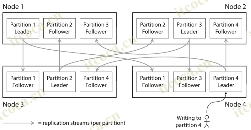
• A node may store more than one partition. If a leader–follower replication model is used, the combination of partitioning and replication can look like this: each partition’s leader is assigned to one node, and its followers are assigned to other nodes

2. Partitioning of Key-Value Data

• Assume that you have a simple key-value data model, in which you always access a record by its primary key

2.1. Partitioning by Key Range

• One way of partitioning is to assign a continuous range of keys (from some minimum to some maximum) to each partition, like the dictionary. If you know the boundaries between the ranges, you can easily determine which partition contains a given key. If you also know which partition is assigned to which node, then you can make your request directly to the appropriate node
• The ranges of keys are not necessarily evenly spaced, because your data may not be evenly distributed. In order to distribute the data evenly, the partition boundaries need to adapt to the data (e.g. A-B, T-Z). The partition boundaries might be chosen manually by an administrator, or the database can choose them automatically
• Within each partition, we can keep keys in sorted order. This has the advantage that range scans are easy, and you can treat the key as a concatenated index in order to fetch several related records in one query. The downside of key range partitioning is that certain access patterns can lead to hot spots (e.g. timestamp), some partition can be overloaded with writes while others sit idle. To avoid this problem, we need to reconsider the choice of key

2.2. Partitioning by Hash of Key

• Because of this risk of skew and hot spots, many distributed datastores use a hash function to determine the partition for a given key. A good hash function takes skewed data and makes it uniformly distributed. For partitioning purposes, the hash function need not be cryptographically strong (such as MD5 and Fowler–Noll–Vo function). Many programming languages have simple hash functions built in, but they may not be suitable for partitioning: for example, in Java’s Object.hashCode() and Ruby’s Object#hash, the same key may have a different hash value in different processes
• Once you have a suitable hash function for keys, you can assign each partition a range of hashes (rather than a range of keys), and every key whose hash falls within a partition’s range will be stored in that partition. This technique is good at distributing keys fairly among the partitions. The partition boundaries can be evenly spaced, or they can be chosen pseudorandomly (sometimes known as consistent hashing). However, by using the hash of the key for partitioning, we lose the ability to do efficient range queries, so that range query has to be sent to all partitions
• Cassandra achieves a compromise between the two partitioning strategies. A table in Cassandra can be declared with a compound primary key consisting of several columns. Only the first part of that key is hashed to determine the partition, but the other columns are used as a concatenated index for sorting the data in Cassandra’s SSTables. A query therefore cannot search for a range of values within the first column of a compound key, but if it specifies a fixed value for the first column, it can perform an efficient range scan over the other columns of the key
• The concatenated index approach enables an elegant data model for one-to-many relationships. For example, on a social media site, one user may post many updates. If the primary key for updates is chosen to be (user_id, update_timestamp), then you can efficiently retrieve all updates made by a particular user within some time interval, sorted by timestamp

• Consistent hashing is a way of evenly distributing load across an internet-wide system of caches such as a content delivery network (CDN). It uses randomly chosen partition boundaries to avoid the need for central control or distributed consensus. Note that consistent here has nothing to do with replica consistency or ACID consistency, but rather describes a particular approach to rebalancing
• This particular approach actually doesn’t work very well for databases, so it is rarely used in practice (the documentation of some databases still refers to consistent hashing, but it is often inaccurate). Because this is so confusing, it’s best to avoid the term consistent hashing and just call it hash partitioning instead

2.3. Skewed Workloads and Relieving Hot Spots

• Hashing a key to determine its partition can help reduce hot spots. However, it can’t avoid them entirely. For example, on a social media site, a celebrity user with millions of followers may cause a storm of activity when they do something. This event can result in a large volume of reads and writes to the same key (where the key is perhaps the user ID of the celebrity, or the ID of the action that people are commenting on)
• Today, most data systems are not able to automatically compensate for such a highly skewed workload, so it’s the responsibility of the application to reduce the skew. For example, if one key is known to be very hot, a simple technique is to add a random number to the beginning or end of the key. Just a two-digit decimal random number would split the writes to the key evenly across 100 different keys, allowing those keys to be distributed to different partitions
• However, having split the writes across different keys, any reads now have to do additional work, as they have to read the data from all 100 keys and combine it. This technique also requires additional bookkeeping: it only makes sense to append the random number for the small number of hot keys; for the vast majority of keys with low write throughput this would be unnecessary overhead. Thus, you also need some way of keeping track of which keys are being split

3. Partitioning and Secondary Indexes

• A secondary index usually doesn’t identify a record uniquely but rather is a way of searching for occurrences of a particular value, such as find all red cars. The problem with secondary indexes is that they don’t map neatly to partitions. There are two main approaches to partitioning a database with secondary indexes: document-based partitioning and term-based partitioning
• Secondary indexes are the bread and butter of relational databases, and they are common in document databases too. Many key-value stores (such as HBase and Voldemort) have avoided secondary indexes because of their added implementation complexity, but some (such as Riak) have started adding them because they are so useful for data modeling. And finally, secondary indexes are the raison d’être of search servers such as Solr and Elasticsearch

3.1. Partitioning Secondary Indexes by Document

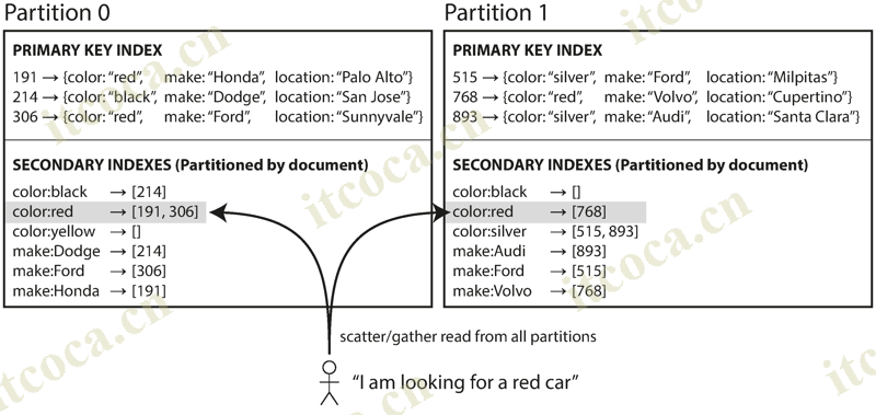
• In this indexing approach, each partition is completely separate: each partition maintains its own secondary indexes, covering only the documents in that partition. It doesn’t care what data is stored in other partitions. Whenever you need to write to the database, you only need to deal with the partition that contains the document ID that you are writing. For that reason, a document-partitioned index is also known as a local index
• However, if you want to search by secondary indexes, you need to send the query to all partitions, and combine all the results you get back. This approach to querying a partitioned database is sometimes known as scatter/gather, and it can make read queries on secondary indexes quite expensive. Even if you query the partitions in parallel, scatter/gather is prone to tail latency amplification. Nevertheless, it is widely used

3.2. Partitioning Secondary Indexes by Term

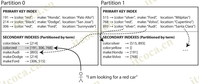
• Rather than each partition having its own secondary index, we can construct a global index that covers data in all partitions. A global index must also be partitioned, but it can be partitioned differently from the primary key index. We call this kind of index term-partitioned, because the term we’re looking for determines the partition of the index. Here, a term would be color:red, for example. The name term comes from full-text indexes (a particular kind of secondary index), where the terms are all the words that occur in a document
• We can partition the index by the term itself, or using a hash of the term. Partitioning by the term itself can be useful for range scans, whereas partitioning on a hash of the term gives a more even distribution of load. The advantage of a global index over a local index is that it can make reads more efficient, without the need to scatter/gather over all partitions. However, the downside is that writes are slower and more complicated, because a write to a single document may now affect multiple partitions of the index
• In an ideal world, the index would always be up to date, and every document written to the database would immediately be reflected in the index. However, in a term-partitioned index, that would require a distributed transaction across all partitions affected by a write, which is not supported in all databases
• In practice, updates to global secondary indexes are often asynchronous (that is, if you read the index shortly after a write, the change you just made may not yet be reflected in the index). For example, Amazon DynamoDB states that its global secondary indexes are updated within a fraction of a second in normal circumstances, but may experience longer propagation delays in cases of faults in the infrastructure

References

• Designing Data-Intensive Application